Time Series Data Wrangling, Exploration, and Visualization

Attaching all relevant packages

library(tidyverse)
library(janitor)
library(lubridate)
library(here)
library(paletteer)
library(tsibble)
library(fable)
library(fabletools)
library(feasts)
library(forecast)
library(sf)
library(tmap)
library(mapview)
library(paletteer)
library(knitr)
library(scales)
library(dplyr)

Reading in the data

salmon <- read_csv("steelhead.csv") %>% 
  clean_names() #Reading in the original observations document and coming up with a data frame 

salmon

Exploring the data

names(salmon) #Names tells you what different variables exist within the entire data set 
unique(salmon$unit) #Unique tells you what different variables exist within the column 
unique(salmon$location) #Unique tells you what different variables exist within the column
unique(salmon$year) #Unique tells me the number of years from 1939 - 2019 

Cleaning up the data

clean_salmon <- salmon %>% 
  mutate(datatype = str_to_lower("datatype")) %>% 
  mutate(parameter = str_to_lower("parameter"))

clean_salmon

Useful descriptive summary of what is included in the data (3-4 sentences)

#This dataset concerns the number of adult passage steelhead salmon (Oncorhynchus mykiss) in the Columbia River Basin at Bonneville Dam from the 1st of January to the 31st of December from 1939 - 2019. The data was collected by the Columbia Basin Research (CBR) research center through the School of Aquatic and Fishery Sciences at the University of Washington under the joint leadership of Research Professor James Anderson and Professor of Biological Statistics John Skalski (Columbia River DART, Columbia Basin Research, University of Washington. (2019). 

Finalized time series plot of original observations for Jan 1st - Jan 31st of 2019

Filtering the dataset

#Need to filer dataset to only display data for 2019 within the month of January from Jan 1st - Jan 31st 

salmon_filtered <- clean_salmon %>%  
 filter(year == 2019) 

salmon_filtered <- clean_salmon %>%  
  filter(month == "Jan")

view(salmon_filtered)

Creating a time series plot of the original observations from January 1st - January 31st, 2019

#Creating a time series plot using ggplot 
steelhead_gg <- ggplot(data = salmon_filtered, aes(x = mm_dd, y = value, group = location)) +
  geom_line(aes(color = year)) +
  theme_minimal() +
  scale_y_continuous(limits = c(0, 30)) + 
  scale_x_discrete(labels=salmon_filtered$mm_dd)  + 
  theme(axis.text.x=element_text(angle=90,size = rel(1.0), margin = margin(1, unit = "cm"),vjust =1)) + 
  labs(x = "January 1st - January 31st 2019 ") + 
  labs(y = "Frequency of daily counts of adult passage \n steelhead salmon (Oncorhynchus mykiss)") + 
  labs(title = "Steelhead salmon (Oncorhynchus mykiss) daily counts \n from Jan 1st - Jan 31st 2019 at Bonneville Dam") + 
  labs(caption = "Steelhead salmon (Oncorhynchusmykiss) daily count \n from Jan 1st - Jan 31st 2019 at Bonneville Dam \n (Columbia River DART, Columbia Basin Research, University of Washington. (2019)") + 
  theme(legend.position = "none") + 
  theme(plot.caption=element_text(hjust=0.5)) + 
  theme(plot.title=element_text(hjust=0.5))

steelhead_gg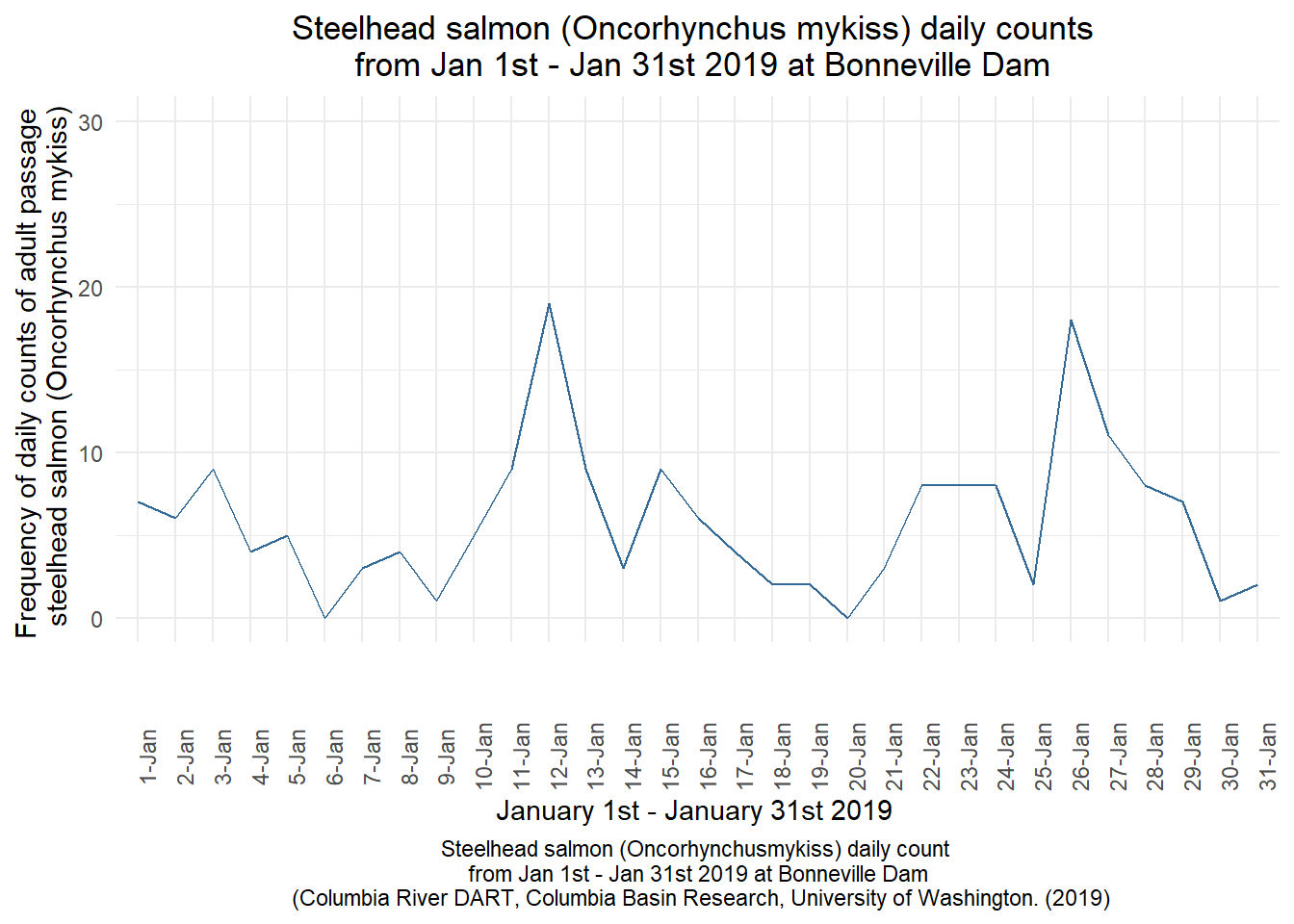

According to the time series plot, the number of daily counts of adult passage steelhead salmon vary depending on the day in January in the year of 2019. The highest daily count was recorded on January 12th with 19 steelhead where as the lowest daily count was recorded on January 6th and January 20th.

Finalized seasonplot of monthly passage

Reading in the data

salmontotal <- read_csv("steelheadtotal.csv")%>%  
  clean_names() #Reading in a new document that contains the month, year, and total daily counts of the dataset 

salmontotal

Creaing the seasonplot of monthly passage in 2019

Creating a new data column in an already existing dataset

#Creating a new data column with the months of 2019 set as factors in order for them to be ordered properly in the graph for ggplot
salmontotal$Month <- factor(salmontotal$month, levels = c("January", "February", "March", "April", "May", "June", "July", "August", "September", "October", "November", "December"))

Creating the seasonplot

#Creating a seasonplot with the total daily counts of the dataset with months on the x axis and total daily counts on the y axis    
ggplot(data = salmontotal, aes(x = Month, y = total, group = year)) + 
  geom_line(aes(color = year)) +
  theme_minimal() +
  theme(axis.text.x=element_text(angle=45,size = rel(1.0), margin = margin(1, unit = "cm"),vjust =1)) + 
  labs(x = "January - December 2019 ") + 
  labs(y = "Frequency of total counts of adult passage \n steelhead salmon (Oncorhynchus mykiss)") + 
  labs(title = "Steelhead salmon (Oncorhynchus mykiss) total counts \n from January - December 2019 at Bonneville Dam") + 
  labs(caption = "Steelhead salmon (Oncorhynchusmykiss) total count \n from January - December 2019 at Bonneville Dam \n (Columbia River DART, Columbia Basin Research, University of Washington. (2019)") + 
  theme(legend.position = "none") + 
  theme(plot.caption=element_text(hjust=0.5)) + 
  theme(plot.title=element_text(hjust=0.5))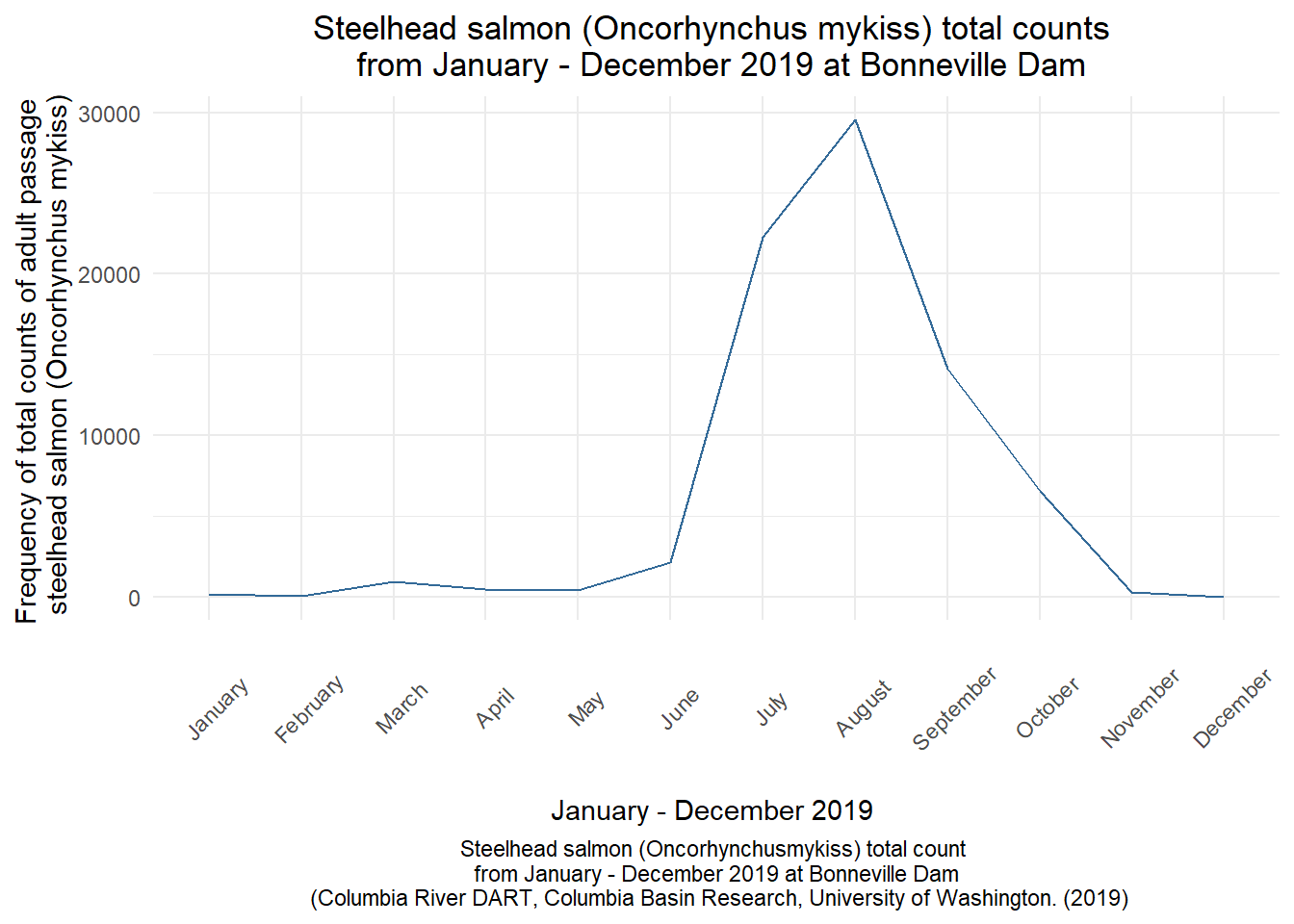

According to the season plot, the number of total counts of steelhead salmon peaks near 30,000 in August 2019. The entire peak area extends on a monthly basis from June - November. It is worth noting that November - May remains relatively the same in terms of total counts of steelhead counts.

Finalized visualization of annual steelhead passage counts

Reading in the data

salmonannual <- read_csv("steelheadannual.csv") #Reading in a new document that contains total steelhead passage data from 2000-2019  

salmonannual

Creating the finalized visualization of the annual steelhead passage counts from 2000 - 2019

#Creating the finalized visualization of annual steelhead passage counts with a barplot
salmon_num <- as.numeric(as.vector(salmonannual$year)) 
salmon_plot <- ggplot(data = salmonannual, aes(x = salmon_num, y = total_daily_count, color = "blue", fill=rgb(0.2, 0.3, 0.5))) + 
  geom_bar(stat="identity") + 
  theme(legend.position="none") + 
  scale_y_continuous(label=comma, limits=c(0, 650000)) + 
  labs(x = "Years of 2000 - 2019") + 
  labs(y = "Frequency of total counts of adult passage \n steelhead salmon (Oncorhynchus mykiss)") + 
  labs(title = "Steelhead salmon (Oncorhynchus mykiss) total counts \n from 2000-2019 at Bonneville Dam") + 
  labs(caption = "Steelhead salmon (Oncorhynchusmykiss) total count \n from 2000-2019 at Bonneville Dam \n (Columbia River DART, Columbia Basin Research, University of Washington. (2019)") + 
  theme(legend.position = "none") + 
  theme(plot.caption=element_text(hjust=0.5)) + 
  theme(plot.title=element_text(hjust=0.5))
  
options(scipen=999) #Resetting the y axis scale to avoid scientific notation and place commas on the y axis. 

salmon_plot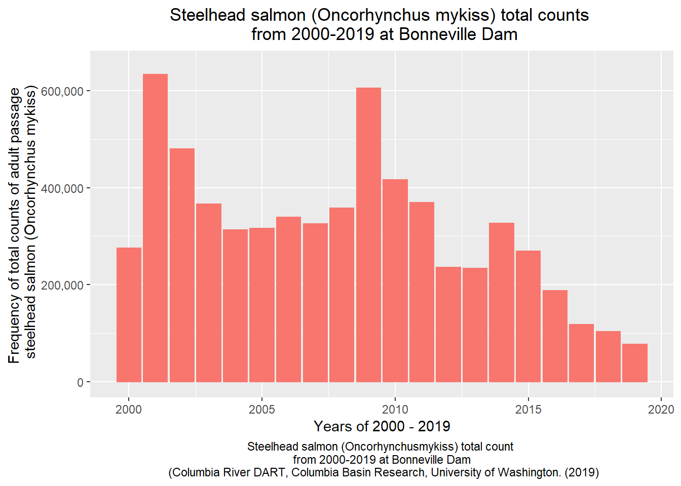

According to the barplot, the number of total counts of adult passage steelhead salmon peaked in 2001 with a grand total of 633,073 counts. There is an interesting cyclical pattern between the years of 2001 - 2009, however, after 2010 the cyclical pattern stops short and instead exhibits a general decreasing trend over time. The lowest year of total counts of adult passage steelhead salmon was in 2019.