
By Nathaniel Burola | March 1, 4040
Data wrangling and visualization with snowshoe hares (Lepus americanus)
Snowshore hares, otherwise known as Lepus americanus, are a keystone prey species that play an ecologically important role in northern boreal forests and experience population fluctuations of 8-11 years. This capture-recapture study of snowshoe hares was conducted at 5 locales in the Tanana valley from study sites Tok in the east to Clear in the west from 1999-2012 with a time duration of 13 years. Snowshoe hare population densities were the highest in 1999 and declined thereafter. This study did not find any declines in apparent survival during declining densities in these study populations.
Attaching all relevant packages
library(tidyverse)
library(janitor)
library(here)
library(kableExtra)
library(naniar)
library(skimr)
library(ggfortify)
library(tmap)
library(ggplot2)
library(hrbrthemes)
library(qwraps2)
library(magrittr)
library(factoextra)
Reading in the data to form a new dataframe
snowshoe <- read_csv("showshoe_lter.csv")Data exploring and wrangling
summary(snowshoe) #Gives a summary of how many different variables there are in the dataframe
View(snowshoe) #Opens a new dataframe with the dataset already in it
names(snowshoe) #Gives the number of column headers in the data set
head(snowshoe) #Gives a preview of the data set
tail(snowshoe) #Gives a preview of the data set

#Initial reaction: Columns that include NA data are the following: time, right ear, sex, age, hindfoot, and notes.

#What variables may be related to each other with this data? Could include sex, age, and weight. Maybe grid and date?

#What do you want to graph with the snowshoe data?

#Statement: I want to see how the weight of all the snowshoe hares both female and male will vary across the years of the study
Filtering and constructing a new dataframe with desired variables
snowfiltered = subset(snowshoe, select = -c(time, grid, trap, l_ear, r_ear, hindft, notes, b_key, session_id, study)) #Filtered out all the columns that are not desired in the new dataframe

#Transforming all of the classes of the variables from character to numeric
Filtering the dataset
#Filtering the dataset in order to get lower case letters for male and females and filtering out the rest of the NA values
snow_tidy <- snowfiltered %>%
  filter(sex %in% c ("f", "m", "M", "F")) %>%
  mutate(
    sex = case_when(
      sex == "f" ~ "F",
      sex == "m" ~ "M")) %>%
  filter(sex!= "NA")
Descriptive introductory summary of what the project is all about (3-4 sentences)
#Snowshore hares, otherwise known as Lepus americanus, are a keystone prey species that play an ecologically important role in northern boreal forests and experience population fluctuations of 8-11 years. This capture-recapture study of snowshoe hares was conducted at 5 locales in the Tanana valley from study sites Tok in the east to Clear in the west from 1999-2012 with a time duration of 13 years. Snowshoe hare population densities were the highest in 1999 and declined thereafter. This study did not find any declines in apparent survival during declining densities in these study populations. Finalized graph about the Bonanza Creek snowshoe hare population
#Creating a histogram based on the weight of the snowshore hares with a frequency count of the data split between by sex (male/female)
snow_plot <- ggplot(snow_tidy, aes(x=weight, color=sex, fill=sex)) +
  geom_histogram(position="identity", alpha=0.5, brewerPalette="Paired",alpha=0.5) +
  labs(title="Weight Distribution of Female and Male Snowshoe Hares from 1999 - 2012",x="Weight (g)", y = "Frequency Count of Snowshoe Hares", caption = "Weight distribution of male and female snowshoe hares (Lepus americanus) \n in Bonanza Creek Experimental Forest (1999-2012) \n (Source: Knut, Kielland, et al. “ Snowshoe Hare Physical Data in Bonanza Creek Experimental Forest: 1999-2012.” Bonanza Creek Experimental Forest, 10 Feb. 2017.") +
  theme_bw()

snow_plot+theme(plot.caption=element_text(hjust=0.5))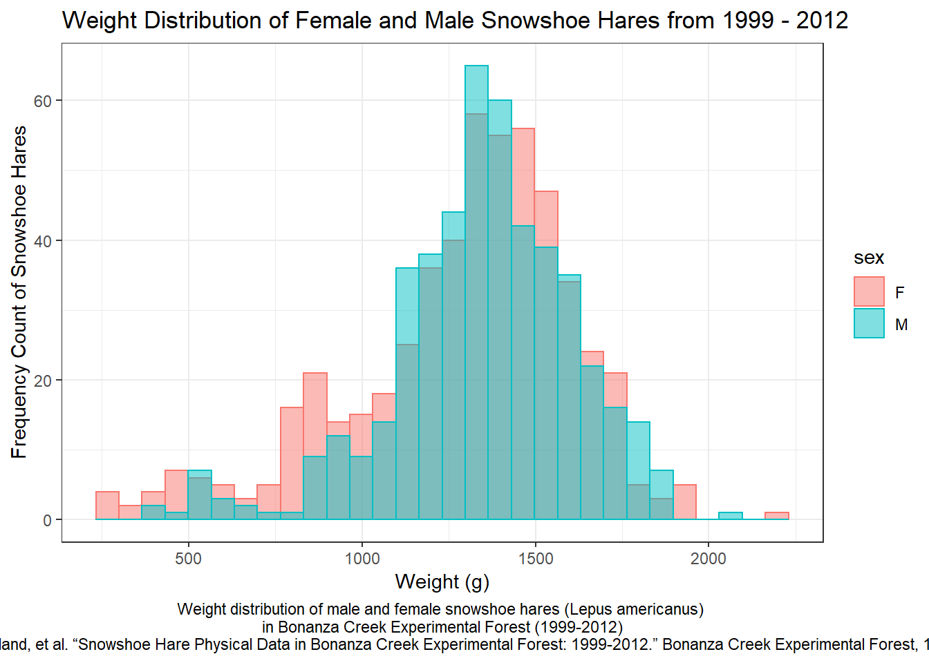
There is a wide range of weights associated with either gender of the snowshoe hare population in Bonanza Creek from 1999-2012. However, there are noticeable differences between male and female snowshoe hares. It would seem that overall there were more male snowshoe hares that weighed in the 1,100 - 1,400 gram range than compared to female snowshoe hares.
Creating a new data frame with desirable traits
#Creating a new data frame to include variables that cannot be analyzed in the numeric class
snowtable = subset(snowshoe, select = -c(time, grid, trap, l_ear, session_id, study, notes, b_key, age, r_ear, hindft))

#Renaming columns in the dataframe to be capitalized
names(snowtable)[names(snowtable) == "sex"] <- "Sex"
names(snowtable)[names(snowtable) == "date"] <- "Year of Study"
names(snowtable)[names(snowtable) == "weight"] <- "Weight of Hare (g)"


#Filtering out the NA values for the new data frame to only get male and female
snow_analysis <- snowtable %>%
  filter(Sex %in% c ("f", "m", "M", "F")) %>%
  mutate(
    Sex = case_when(
      Sex == "f" ~ "F",
      Sex == "m" ~ "M")) %>%
  filter(Sex!= "NA")

#Filtering out female snowshow hares to only get the males for data analysis results
snow_male <- snow_analysis %>%
 filter(Sex!= "F")

snow_male

#Filtering out male snowshow hares to only get the females for data analysis results
snow_female <- snow_analysis %>%
 filter(Sex!= "M")

snow_female
Testing out various statistical analyses
#Calculating Descriptive Statistics of the Weight of Female Snowshoe Hares
mean(snow_female$`Weight of Hare (g)`, na.rm = TRUE)
#1289.994
median(snow_female$`Weight of Hare (g)`, na.rm = TRUE)
#1350
sd(snow_female$`Weight of Hare (g)`, na.rm = TRUE)
#325.08004
min(snow_female$`Weight of Hare (g)`, na.rm = TRUE)
#240
max(snow_female$`Weight of Hare (g)`, na.rm = TRUE)
#2170
range(snow_female$`Weight of Hare (g)`, na.rm = TRUE)
#1930
Creating the finalized HTML table
snow_tbl <- data.frame(
  Statistics = c("Mean", "Median", "Standard Deviation", "Minimum", "Maximum", "Range"),
  Calculations = c(
    "1,290 ",
    "1,350",
    "325 ",
    "240",
    "2,170",
    "1,930"
  )
)

kable(snow_tbl, caption = '<b>Female Snowshoe Hare Weight Descriptive Statistics</b>') %>%
  kable_styling(full_width = F) %>%
  column_spec(1, bold = T, border_right = T) %>%
  column_spec(2, width = "30em", background = "white") %>%
footnote(general = "Descriptive statistics which calculate the mean to range of weights for all female snowshoe hare populations in Bonanza Creek Experimental Forest (1999-2012)") | Statistics | Calculations |
|---|---|
| Mean | 1,290 |
| Median | 1,350 |
| Standard Deviation | 325 |
| Minimum | 240 |
| Maximum | 2,170 |
| Range | 1,930 |
| Note: | |
| Descriptive statistics which calculate the mean to range of weights for all female snowshoe hare populations in Bonanza Creek Experimental Forest (1999-2012) |
According to the data, female snowshoe hare populations from 1999-2012 in Bonanza Creek have a mean weight of 1,290 grams and a median weight of 1,350 grams. The lightest female snowshoe hare weighed 240 grams while the heaviest female snowshoe hare weighed 2,170 grams. Taking into account the entire female population, there was a range of 1,930 grams from the lightest to the heaviest female snowshoe hare. The standard deviation of the female snowshoe population was 325 grams in relation to the mean weight of 1,290 grams.
Principal components analysis (PCA)
What humans eat in terms of their food supply and the scientiifc understanding of relationships between dietary intakes and health have evolved over time. As the United States Department of Agriculture (USDA), this organizations is responsible for maintaining food composition data resources that can meet the needs of diverse users from researchers to health professionals. There is a need for transparent and easily accessible information about nutrients and a new approach to presenting food profile information as the food industry changes over time. This dataset, titled FoodData Central, presents food profile information in a scientifically rigorous way (Source: FoodData Central . “FoodData Central .” FoodData Central, 2020, fdc.nal.usda.gov/about-us.html.)
Reading in the dataset
nutrients <- read_csv("usda_nutrients.csv")Doing some data wrangling to clean up and filter the data
#Filtered the dataset through food group in onder to have vegetables and vegetable products as well as fruits and fruit juices

#Retaining observations where the ShortDescrip column would contain the word "RAW"
usda <- nutrients %>%
  filter(FoodGroup  == "Vegetables and Vegetable Products" |
           FoodGroup == "Fruits and Fruit Juices") %>%
  filter(str_detect(ShortDescrip, pattern="RAW"))
Useful descrptive summary (3-4 lines)
#What humans eat in terms of their food supply and the scientiifc understanding of relationships between dietary intakes and health have evolved over time. As the United States Department of Agriculture (USDA), this organizations is responsible for maintaining food composition data resources that can meet the needs of diverse users from researchers to health professionals. There is a need for transparent and easily accessible information about nutrients and a new approach to presenting food profile information as the food industry changes over time. This dataset, titled FoodData Central, presents food profile information in a scientifically rigorous way (Source: FoodData Central . “FoodData Central .” FoodData Central, 2020, fdc.nal.usda.gov/about-us.html.) Creating the summary table for the PCA analysis
## Importance of components:
##                           PC1    PC2     PC3    PC4     PC5     PC6     PC7
## Standard deviation     2.3112 1.5885 1.37202 1.3349 1.14690 1.04587 1.01824
## Proportion of Variance 0.2428 0.1147 0.08557 0.0810 0.05979 0.04972 0.04713
## Cumulative Proportion  0.2428 0.3575 0.44306 0.5241 0.58385 0.63357 0.68070
##                            PC8     PC9    PC10    PC11    PC12    PC13    PC14
## Standard deviation     0.95692 0.92741 0.89055 0.82930 0.75584 0.70965 0.68029
## Proportion of Variance 0.04162 0.03909 0.03605 0.03126 0.02597 0.02289 0.02104
## Cumulative Proportion  0.72232 0.76142 0.79747 0.82873 0.85470 0.87759 0.89862
##                           PC15    PC16    PC17   PC18    PC19    PC20    PC21
## Standard deviation     0.63747 0.58068 0.57007 0.5609 0.50314 0.48474 0.44798
## Proportion of Variance 0.01847 0.01533 0.01477 0.0143 0.01151 0.01068 0.00912
## Cumulative Proportion  0.91709 0.93242 0.94719 0.9615 0.97300 0.98368 0.99280
##                          PC22
## Standard deviation     0.3980
## Proportion of Variance 0.0072
## Cumulative Proportion  1.0000
Creating the finalized PCA plot
usda_bilplot <- autoplot(usda_pca,
                       colour = NA,
                       loadings.label = TRUE,
                       loadings.label.size = 3,
                       loadings.label.colour = "black",
                       loadings.label.repel = TRUE) +
   labs(title = "PCA Biplot: Fruit and Vegetable Nutrient Levels",
       x = "PC1 representing 24.80% of variance",
       y = "PC2 representing 11.47% of variance",
       caption = "PCA biplot representing fruit and vegetable nutrient levels \n including variables from protein (g) to zinc levels \n (Source: Food Data Central .“FoodData Central .” FoodData Central, 2020, fdc.nal.usda.gov/about-us.html.") +
  theme_bw()

usda_bilplot + theme(plot.caption=element_text(hjust=0.5)) + theme(plot.title=element_text(hjust = 0.5))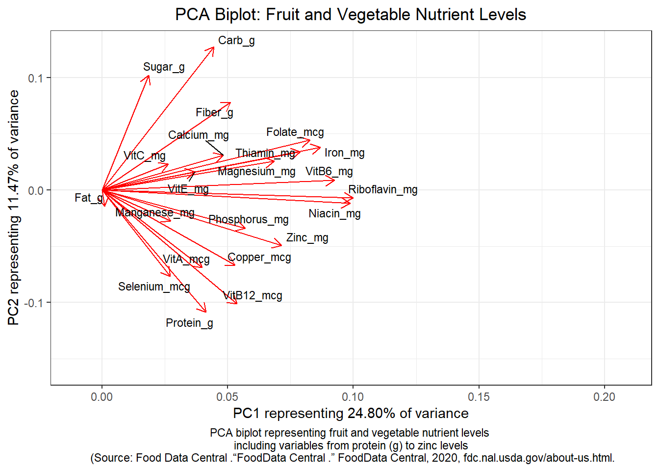
The PCA biplot can be interpreted in multiple trends:
Postive Trend: In terms of postive correlation, Riboflavin and Niacin are postively correlated with one another on account of the length and overlap of their biplot lines. Magnesium and Thiamin are postively correlated with each other as well as Iron and Folate. Sugar and Carbs are postively correlated with one another since they are still in close proximity to one another with their biplot lines.
Negative Trend: In terms of negative correlation, Sugar and Protein are negatively correlated due to the 180 degree difference between biplot lines earning a correlation of -1. Sugar and Selenium also appear to be negatively correlated as well.
Neutral Trend: In terms of minimal or no correlation, Sugar and Manganese are minimally correlated with one another due to the 90 degree difference of their biplot lines. Sugar and Fat have minimal or no correlation at all since there is a 270 degree difference between the two biplot lines.