
By Nathaniel Burola | March 1, 4040
Chlorophyll Concentrations Along The California Coast (2016)
This project details chlorophyll concentrations along the California coast, specfically in locations such as Stearns Wharf in Santa Barbara. Concentrations were analyzed with the month, median, maximum, mean, standard deviation, and sample size in mind. The significant difference of harmful algal blooms observed in Cal Poly Pier and Stearns Wharf was calculated using statistical tests such as the F-Test studying an F-distribution under the null hypothesis as well as a two sample T-Test along with Cohen’s D which looks at effect sizes. Overall, there was a significant difference in harmful algal blooms between the two locations.
Loading necessary packages
suppressPackageStartupMessages({
  library(tidyverse)
  library(dplyr)
  library(pwr)
  library(knitr)
  library(kableExtra)
  library(plotly)
  library(ggrepel)
  library(extrafont)
  library(tinytex)
  library(RColorBrewer)
  library(ggpubr)
  library(effsize)
})
Loading the dataset into R
hab <- read_csv("hab.csv")## Parsed with column specification:
## cols(
## year = col_double(),
## month = col_double(),
## location = col_character(),
## chlorophyll = col_double(),
## temp = col_double()
## )hab #Viewing the new dataset in a new frame Finalized table of the median, maximum, mean, standard deviation, and sample size for chlorophyll concentrations at Stearns Wharf By month in 2016
Creating a summary table with the month, median, maximum, mean, standard deviation, and sample size for chlorophyll concentrations
#Creating the summary table with the month, median, maximum, mean, standard deviation, and sample size for chlorophyll concentration

summary_chlorophyll <- hab %>%
  filter(year == 2016,
         location == "Stearns Wharf",
         chlorophyll != "Nan") %>%
  select(year:chlorophyll) %>%
  group_by(month) %>%
  summarise(
    Median = round(median(chlorophyll), digits = 2),
    Maximum = round(max(chlorophyll), digits = 2),
    Mean = round(mean(chlorophyll), digits = 2),
    `Standard Deviation` = round(sd(chlorophyll), digits = 2),
    `Sample Size` = length(chlorophyll))

summary_chlorophyll #Viewing the summary table for the chlorophyll information
Rewriting the numerical values of the month column and creating an upgraded summary table
#Rewriting the numerical values of the month column to reflect the names of the months of the year starting from January ("Jan") to December ("Dec")

summary_chlorophyll2 <- summary_chlorophyll %>%
  mutate(
    Month = case_when(
      month == 1 ~ "Jan",
      month == 2 ~ "Feb",
      month == 3 ~ "Mar",
      month == 4 ~ "Apr",
      month == 5 ~ "May",
      month == 6 ~ "Jun",
      month == 7 ~ "Jul",
      month == 8 ~ "Aug",
      month == 9 ~ "Sep",
      month == 10 ~ "Oct",
      month == 11 ~ "Nov",
      month == 12 ~ "Dec")) %>%
  select(Month, Median, Maximum, Mean, `Standard Deviation`, `Sample Size`)

summary_chlorophyll2 #Viewing the upgraded version of the summary table for the chlorophyll information with categorical labels for months instead of numerical values
Creating a table for chlorophyll concentrations
#Creating a table for chlorophyll concentrations using the kable function with month, median, maximum, mean, standard deviation, and sample size values
table_chlorophyll <- kable(summary_chlorophyll2,
                           caption = "Table 1: Chlorophyll Concentrations (mg/m^3^) from January 2016 - December 2016 at Stearns Wharf, Santa Barbara",
               booktabs = T) %>%
  kable_styling(bootstrap_options = c("striped", "hover", "condensed", "responsive", "hold_position"), full_width = FALSE, position = "center")

table_chlorophyll #Viewing the table in a new frame | Month | Median | Maximum | Mean | Standard Deviation | Sample Size |
|---|---|---|---|---|---|
| Jan | 2.27 | 3.32 | 2.31 | 0.83 | 4 |
| Feb | 1.12 | 1.59 | 1.00 | 0.45 | 5 |
| Mar | 0.95 | 1.27 | 0.92 | 0.39 | 4 |
| Apr | 1.22 | 3.89 | 1.78 | 1.45 | 4 |
| May | 3.54 | 9.54 | 4.35 | 3.12 | 5 |
| Jun | 2.34 | 4.21 | 2.56 | 1.24 | 4 |
| Jul | 1.15 | 1.77 | 1.21 | 0.44 | 4 |
| Aug | 2.10 | 5.42 | 2.65 | 1.60 | 5 |
| Sep | 2.33 | 2.78 | 2.09 | 0.81 | 4 |
| Oct | 2.24 | 3.93 | 2.46 | 0.85 | 5 |
| Nov | 0.88 | 2.54 | 1.22 | 0.90 | 4 |
| Dec | 2.53 | 4.60 | 2.75 | 1.36 | 4 |
Finalized column graph of the mean monthly chlorophyll concentration at Stearns Wharf, Santa Barbara in 2016
Creating a column graph of mean monthly chlorophyll concentrations at Stearns Wharf in 2016
#Creating a column graph of the mean monthly chlorophyll concentration at Stearns Wharf in 2016 from the summar table that was created in Question 1
column_chlorophyll <- ggplot(summary_chlorophyll2, aes(x=Month, y=Mean)) +
    geom_col(aes(fill = Month), show.legend = FALSE, position=position_dodge()) +
    geom_errorbar(aes(ymin=Mean-`Standard Deviation`, ymax=Mean+`Standard Deviation`),
                  width=.2,
                  position=position_dodge(.9))  +
  labs(x = "Month",
       y = expression ('Mean Chlorophyll Concentration ± 1 SD (mg/m'^3*')')) +
       scale_y_continuous(expand = c(0,0), limits = c(0,8))+
       ggtitle("Mean Chlorophyll Concentration at Stearns Wharf Per Month in 2016 \nNathaniel Burola \n")+
   scale_fill_brewer(palette = "Paired")  +
  scale_x_discrete(limits = month.abb)

column_chlorophyll #Viewing the column graph in a new frame 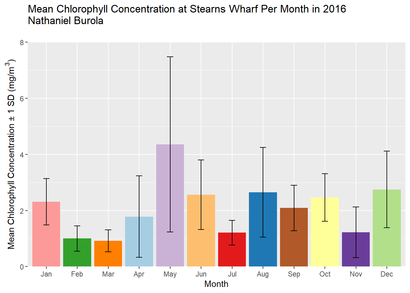
Figure 1: Mean monthly chlorophyll concentrations (mg/m3) at Stearns Wharf, Santa Barbara measured from January 2016 to Dececmber 2016 with black error bars. Said error bars represent standard deviation which in this case is ±1 standard deviations away from the mean chlorophyll concentration for a given month.
Calculating long-term algal bloom threats
Identifying questions and writing down the null and alternative hypotheses
#Identify question: "Does the yearly chlorophyll average at a site exceed 2.0mg/m3"?
#Type of significance test that we need to run is a one-sample, one-tailed T-Test

#Null Hypothesis (H0): The yearly chlorophyll average for 2016 is not greater than the long term limit of 2.0mg/m3
#Alternative Hypothesis (HA): The yearly chlorophyll average for 2016 is greater than the long term limit of 2.0mg/m3
Creating a new data table with filtered values
#Creating a new data table with filtered values for monthly chlorophyll concentrations pertaining only to Stearns Wharf in 2016.
algae_threat <- hab %>%
  filter(location == "Stearns Wharf",
         year == 2016,
         chlorophyll !="NAN") %>%
  select(-temp)

algae_threat #Viewing the data table in a new frame
Calcuating the mean and standard deviation (SD) of chlorophyll concentrations for Stearns Wharf
algae_mean <- mean(algae_threat$chlorophyll)
algae_sd <- sd(algae_threat$chlorophyll)

algae_mean #Viewing the mean result for Stearns Wharf
algae_sd #Viewing the standard deviation result for Stearns Wharf
Calculating a one sample, one-sided T-Test for Stearns Wharf
#Performing the one-sample, one-sided T-Test for Stearns Wharf with the alternative labelled as "greater"
algae_oneside <- t.test(algae_threat$chlorophyll, alternative = c("greater"), mu =2)

algae_oneside #Viewing the one-sample, one-sided T-Test for Stearns Wharf

#p value of 0.2518 and is greater than the significance level of 0.05 (p > 0.05)
#Sufficient to not dispute (retain) the null hypothesis
Publication Final Statement: If the yearly chlorophyll average at a site exceeds the long-term limit of 2.0mg/m\(^3\), the probability of a long-term algal bloom threat occuring is very likely. After conducting a one-sample, one-sided T-Test, there was sufficient evidence to not dispute the null hypothesis as the yearly chlorophyll average for 2016 at Stearns Wharf, Santa Barbara was not significantly greater than the long-term limit of 2.0mg/m\(^3\) (t(51 = 0.67, p = 0.252, \(\alpha\) = 0.05). It is doubtful that the area of Stearns Wharf in Santa Barbara would be threatened by long-term algal bloom threats in the future.
Calculating the significant difference between Cal Poly Pier and Stearns Wharf
Writing down the research question
#Question: Based on all observations at the two sites in 2016, is there a significant difference in mean annual chlorophyll concentration (an indicator for algal growth) near Cal Poly Pier and Stearns Wharf?

#Need to first do some exploratory data analysis in order to see which statistical analysis test to pursue
Creating a new data table with Stearns Wharf and Cal Poly Pier values for 2016
#Filtering the shellfish data frame by year, location, and removing all chlorophyll Nan values
shellfish <- hab %>%
  filter(year == "2016",
         location == "Stearns Wharf" | location == "Cal Poly Pier",
         chlorophyll != "Nan") %>%
  select(location, chlorophyll)

shellfish #Viewing said table in a new frame
Graph side-by-side histogram to evaluate the normal distribution of the data
shellfish_hist <- ggplot(shellfish, aes(x = chlorophyll)) +
  geom_histogram(aes(fill = location)) +
  facet_wrap(~ location, scale = "free")

shellfish_hist #Viewing said histogram in a new frame
## `stat_bin()` using `bins = 30`. Pick better value with `binwidth`.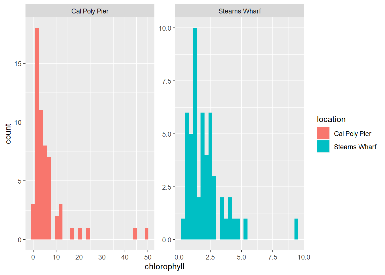
Graph QQ-Plot to evaluate the normal distribution of the data
qqp <- ggplot(shellfish, aes(sample = chlorophyll)) +
  geom_qq(aes(color = location)) +
    facet_wrap(~ location, scale = "free")

qqp #Viewing said qqplot in a new frame 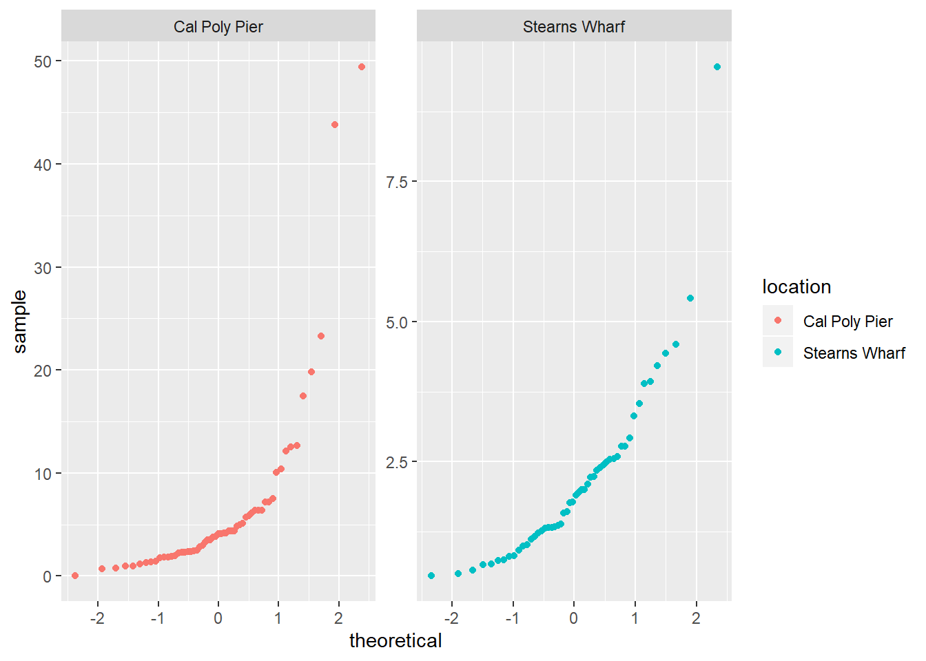
The histogram and the QQ-Plot do not show a normally distributed population and look non-parametric. The histogram does not show normal distribution as there are outliers that prevent a normal distribution curve from being drawn. The QQ-Plot data points do not adhere to a line of linearity. However, the sample size from Table 1 is n=52 (n>30). Keeping in mind the Central Limit Theorem (CLT), it can be assumed that the means in this case will be normally distributed. Seeing as there is no directionality stated, we can utilize a two-sample, two-sided T-Test with a 95% Confidence Interval and a significance level of 0.05. However, it would be better to perform a F-Test for equal variances first just in case we need to override the assumption with (var.equal = FALSE) depending on the result we get concerning the ratio of the variances.
Performing the F-Test for Equal Variances
#Performing the F-Test for Equal Variances

#Null Hypothesis (H0): The ratio of variances between Caly Poly Pier and Stearns Wharf is 1 (there is no difference; the variances are equal)

#Alternative Hypothesis (HA): The ratio of variances between Caly Poly Pier and Stearns Wharf is not equal to 1 (there is a difference; the variances are not equal)
Performing the F-Test
#Performing the F-Test
shellfishf <- shellfish %>%
  var.test(chlorophyll ~ location, data = .)

shellfishf #Viewing the F-Test

#P value is <2.2e-16 and is less than the significance level of 0.05 (p < 0.05)
# If p < 0.05, then we have enough evidence to reject the null hypothesis (accept alternative hypothesis instead)
# As a result, we cannot overwrite the default in the T.Test function (var. equal = FALSE)
Graphing a box and whisker plot with an overlaying jitterplot to visualize the distribution of the data
shellfish_baj <- ggplot(shellfish, aes(x = location, y = chlorophyll)) +
  geom_boxplot() +
  geom_jitter(width = 0.1, aes(color = location)) +
  labs(x = "Location",
       y = expression ('Chlorophyll Concentration (mg/m'^3*')')) +
  theme_classic() +
  guides(colour=FALSE)

shellfish_baj #Viewing said box and whisker plot with an overlaying jitterplot in a new frame 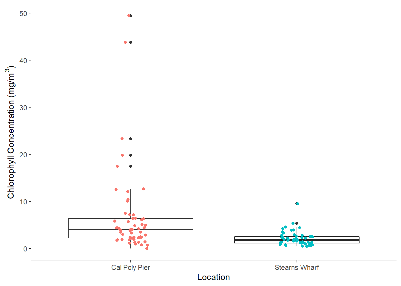
Data appears to be heavily clustered in one spot for Stearns Wharf, however, for Cal Poly Pier, the data appears to be more widespread across the box and whisker plot overlayed with a jitterplot
Writing down hypotheses and confidence intervals
#Assumed 95% Confidence Interval with significance level of 0.05
#Null Hypothesis (H0): The mean annual chlorophyll concentrations (mg/m3) near Stearns Wharf and Cal Poly Pier are equal (no difference in means)

#Alternative Hypothesis (HA): The mean annual chlorophyll concentrations (mg/m3) near Stearns Wharf and Cal Poly Pier are not equal (difference in means)
Conducting the T-Test for Shellfish
shellfishtt <- shellfish %>%
  t.test(chlorophyll ~ location, data = .)

shellfishtt #Viewing the two-sample, two-sided T-Test in a new frame

#Obtained results from a Welch Two Sample T-Test with a p-value of 0.0006082 (p<0.05)
#Sufficient evidence to reject the null hypothesis (H0) and accept the alternative hypothesis (HA)
#Difference in mean annual chlorophyll concentrations (mg/m3) Stearns Wharf and Cal Poly Pier
Evaluating Effect Size with Cohen’s D
#Measure of how many standard deviations apart two means are

#Creating vector for Cal Poly

calpolyd <- shellfish %>%
  filter(location == "Cal Poly Pier") %>%
  pull(chlorophyll)

#Creating vector for Stearns Wharf

stearnsd <- shellfish %>%
  filter(location == "Stearns Wharf") %>%
  pull(chlorophyll)

#Calculating Effect Size with Cohen's D
effectsize <- cohen.d(calpolyd, stearnsd)

effectsize #Viewing said effect size

#Result: Moderate effect size of 0.66
Calculating Absolute Difference Between Means in Stearns Wharf and Cal Poly Pier
#Taking the mean results from the earlier Welch Two Sample T-Test for Cal Poly Pier and Stearns Wharf and subtracting them to get the absolute difference

#Mean in Cal Poly Pier group: 6.55
#Mean in Stearns Wharf group: 2.15
#Absolute Difference: 4.4
Finding the Mean and Standard Deviation of Cal Poly Pier
#Creating a new table with Cal Poly Pier values for 2016
calpolypier <- hab %>%
  filter(year == 2016,
         location == "Cal Poly Pier",
         chlorophyll != "NaN") %>%
  select(year:chlorophyll)

calpolypier #Viewing said data table

#Finding the mean of Cal Poly Pier
cal_mean <- mean(calpolypier$chlorophyll)

cal_mean #Viewing said mean of Cal Poly Pier

#Finding the standard deviation of Cal Poly Pier
cal_sd <- sd(calpolypier$chlorophyll)

cal_sd #Viewing said standard deviation of Cal Poly Pier
Problem 4 Interpretation: While the difference in means of annual chlorophyll concentration near Cal Poly Pier (6.55 mg/m\(^3\) ±9.03) and Stearns Wharf (2.15mg/m\(^3\) ±1.57) is significant (t(59.69 = 3.62, p = 0.001, \(\alpha\) = 0.05), the mean annual chlorophyll concentration for Stearns Wharf (n=52) is statistically less than than the mean annual chlorophyll concentration for Cal Poly Pier (n=57). The effect size between the two means is moderate (Cohen’s D = 0.66) with an absolute difference of 4.44 mg/m\(^3\). Keeping this data in mind, it would be a bad investment to develop any aquaculture project in Cal Poly Pier compared to Stearns Wharf due to the higher probability of a long-term algal bloom.